Rainbow Tables (probably) aren’t what you think — Part 1: Precomputed Hash Chains

Note: To understand this article, you‘ll need to understand password hashing and cracking first. Rainbow Tables are a very interesting but also fairly complex data structure, so if you aren’t interested in CompSci, you probably won’t be into this article.

Rainbow Attack by TheeWeguy

Rainbow Tables != Lookup Tables

Many people use “rainbow table” to refer to “a lookup table of password hashes”, but in reality a rainbow table is a far more complex, and more interesting technology. This article will discuss the problem with lookup tables, and how rainbow tables solve it. We’ll be focusing on a scenario where we want to crack any md5 hash of a 4 digit password, meaning our search space looks like so:

0000
0001
0002
...
9999

Lookup Tables Explained

Lookup tables are probably what you thought rainbow tables are, and are what most people mean when they say “rainbow table”. A lookup table is an extremely simple data structure. All it does is store both the hash and the corresponding password in a massive list. For example, by hashing the candidate list and storing the hash, we arrive at the following list:

4a7d1ed414474e4033ac29ccb8653d9b:0000
25bbdcd06c32d477f7fa1c3e4a91b032:0001
fcd04e26e900e94b9ed6dd604fed2b64:0002
...
fa246d0262c3925617b0c72bb20eeb1d:9999

In reality, you’d sort the file by the hash value, allowing you to use a binary search instead of having to read every line. But that’s not the focus of this article.

Lookup tables are a very simple and elegant solution, and can be searched very quickly, but the storage space quickly becomes infeasible for more complex passwords. For example, if we wanted to create a lookup table for all 8 character passwords with a full upper/lower/digits/symbols character set, we’d need about 160 PetaBytes of storage… Clearly another solution needs to be used at that scale.

Precomputed Hash Chains

The predecessor of rainbow tables, precomputed hash chains allow us to store far less on disk, at the expense of greater computing power requirements at “lookup” time.

To generate a hash chain, we need to first define a reduction function. Whereas a hash function takes a password and converts it into a hex string, our reduction function takes a hex string and converts it into a password within our desired search space. You can think of this as a random password generator that uses the input hash as a seed.

For example, when a hash function behaves like so:

0000 -> 4a7d1ed414474e4033ac29ccb8653d9b

Our reduction function would behave like so:

4a7d1ed414474e4033ac29ccb8653d9b -> 4515

Note that this is not reversing the hash, it’s deriving a new password from the hash. With hash and reduction functions, we can only go forward, never backwards.

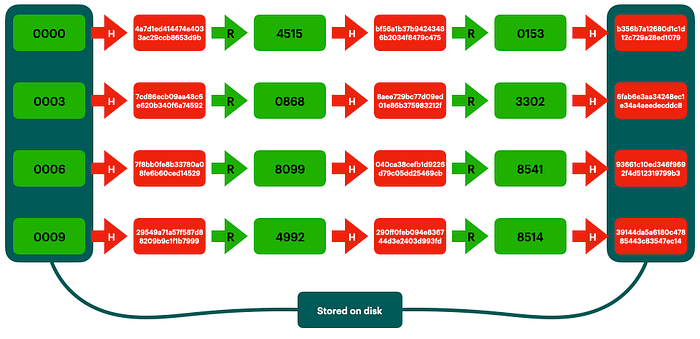
We then use our hash and reduction functions to generate a bunch of hash chains (in this instance each chain is 3 long):

Here’s the clever part. We never store the full hash chain, we only store the first and last link of each chain. As with the lookup tables, we’d probably sort the hash chains by the hash value for quicker lookup, but we’re ignoring that for the sake of illustration. We also need to store some metadata, like the chain length and the reduction function, so that we can recreate individual chains when needed.

It might seem strange that we’re spending the cycles to calculate the hash results but then not actually storing all the results. But here’s a useful way to think about it: Precomputed hash chains don’t store the solutions, they store hints that allow you to do a more targeted brute force at lookup time. Still confused? Keep reading to see how we use the chains.

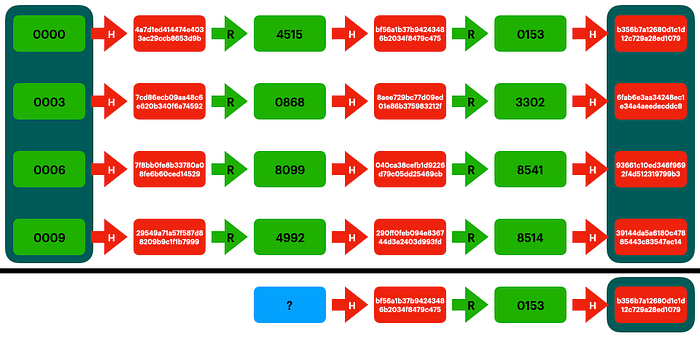
Imagine we have the hash bf56a1b37b94243486b2034f8479c475 and we want to find its corresponding password. We can check if we’ve already computed this before, by following the same process we used to generate the chains. By reducing and hashing, comparing with the saved hashes in the precomputed chains every time, we discover that we previously computed this hash in the 0000 chain.

Now that we know we’ve found the chain containing our solution, we can recreate it from the start to find the input of that solution, and therefore crack our hash.

Like I said before, at no point did we store the solution. Instead, we store a way to figure out if we’ve ever computed the solution before, and a way to reproduce the previous computations in a more targeted way. Instead of having to calculate all 10000 md5 hashes at “lookup time”, we only had to calculate 3 md5 hashes. Likewise, instead of having to store all 10000 results, we’d only had to store ~3333 hashes to cover the full search space.

In other words, we divided our storage factor by our computing factor. This allows us to tune our solution to take advantage of either a large amount of storage allowing cheap lookup, or more expensive lookup with lower storage requirements. Going back to our example of wanting to crack any 8 character md5 hash, we can divide our storage requirements by 100,000 by using precomputed chains of that length. Now we only have to store 1.6 TB of data, and we can crack any hash by computing 100,000 hashes (about 4 microseconds of computation on an RTX 3090) instead of 6,704,780,954,517,120 hashes (2 days of computation on an RTX 3090).

This is a great example of a time/space tradeoff, and is the basis of how rainbow tables work. Honestly, you can probably stop here and have a good understanding of lookup tables vs rainbow tables. However, if you’re like me and really want to know the dirty details, give Part 2 a read.